PostgreSQL Monitoring

PostgreSQL Monitoring

In this post, We will explore how to analyze PostgreSQL performance not just from inside the database, but in tandem with the operating system layer.

We won’t be diving into setting up dashboard thresholds, writing alarm scripts, or creating critical/warning scenarios here. These are vital and if you are not doing them, you are not truly monitoring but they are not the focus of this article. Instead, We will focus on the final visualizations and how to interpret them. We will answer the question: Why does this graph look like this?

Table of Contents

Section 1: Operating System and Infrastructure Health

• 1.1. System Load & CPU Busy: Analyzing the processor queue and actual utilization.
• 1.2. Memory Usage & Swap: RAM capacity management and the performance killer: Swap usage.
• 1.3. Filesystem Usage: Monitoring disk occupancy and preventing crash risks.
• 1.4. Disk Latency (R/W Time) & IOPS: Detecting I/O Wait bottlenecks and data transfer rates.
• 1.5. Network Traffic: Bandwidth limits and network traffic spikes.
• 1.6. OOM Killer Count: Tracking the risk of the OS terminating PostgreSQL processes.
• 1.7. Uptime & Stability: System reliability and continuous operation time.

Section 2: PostgreSQL Engine and Cache Efficiency

• 2.1. PG Buffer Cache Hit Rate: Success rate of accessing data from memory (Why 99%?).
• 2.2. Temp File Usage: Traces of queries that don’t fit in memory and spill to disk.

Section 3: Traffic, Connections, and Timed Risks

• 3.1. Active vs. Idle Sessions: Connection pool management and the need for PgBouncer.
• 3.2. Database Size & Growth: Data growth trends and capacity planning.
• 3.3. Replication Lag: Synchronization health in High Availability (HA) architectures.

Section 4: Bottlenecks, Locks, and Rogue Queries

• 4.1. Longest Transaction & Top Long-Running Queries: Chronic queries slowing down the system.
• 4.2. Lock Tables: Data contention and deadlock analysis.

Section 5: Conclusion and Action Plan

• 5.1. Quick Fixes: 3 steps for instant performance improvement.
• 5.2. Monitoring Strategy: Table of critical alarm thresholds.

Section 1: Operating System and Infrastructure Health

1.1 System Load & CPU Busy: Is the system hanging? Analyzing the processor queue.

When a database slows down, the first instinct is often to blame a specific query. But before diving into SQL, we need to look at the atmospheric pressure of the server: System Load and CPU Busy.

• System Load (Load Average): This represents the number of processes currently using the CPU plus those waiting in the queue.
• The Interpretation: If your 8-core server shows a Load Average of 15, your CPU is oversaturated. Processes are literally standing in line to be processed. This usually points to a “concurrency” issue where the database is trying to do more than the hardware allows.
• CPU Busy (Utilization): This tells us what percentage of the CPU’s total capacity is being used.
• Crucial Insight: High CPU isn’t always a bad thing it means you’re getting your money’s worth from the hardware. The real red flag is I/O Wait. If your CPU is busy simply waiting for the disk to respond, your bottleneck isn’t your processor; it’s your storage.

By analyzing these two metrics together, we can distinguish between a calculation-heavy problem (like a complex mathematical function in SQL) and a waiting problem (like slow disks or locking issues).

This panel measures what percentage of the server’s total processing power is actively being utilized. The analysis is based on a fundamental logic:

• The Logic: The system’s true engagement rate is calculated by subtracting the “idle time” from the total CPU capacity.
• Critical Threshold: If CPU utilization consistently hovers around the 80–90% range, it indicates that the system is hitting a bottleneck and is starting to queue up new operations.

The PromQL Query:

(
  (
    count(count(node_cpu_seconds_total{instance="$node", job="$job"}) by (cpu)) 
    - 
    avg(sum by (mode)(irate(node_cpu_seconds_total{mode='idle', instance="$node", job="$job"}[5m])))
  ) 
  * 100
) 
/ 
count(count(node_cpu_seconds_total{instance="$node", job="$job"}) by (cpu))

Query Components:

• Total Core Count: The count function identifies the number of CPU cores available in the system.
• Instantaneous Change (irate): By using the rate of change over the last 5 minutes, we minimize noise from sudden spikes and get a smoother, more accurate trend.
• Percentage Output: By proportioning the total “busy” time against the core count, we arrive at the specific utilization figure — such as the 9.16% usage shown in the visualization.

This panel measures not just how busy the processor is, but also the density of the task queue and the overall pressure on the system.

• The Logic: System Load (Load Average) represents the CPU cores’ ability to satisfy current demand. If this value is lower than the total core count, the system is fluid. If it exceeds the core count, it means processes are queued up and waiting for their turn.
• Critical Threshold: When this value crosses the 70–80% band relative to total capacity, it serves as a leading indicator that the system is struggling to meet incoming requests and latency will inevitably begin to spike.

The PromQL Query:

(
  node_load5{instance="$node", job="$job"}
  /
  count(count(node_cpu_seconds_total{instance="$node", job="$job"}) by (cpu))
) * 100

Query Analysis: The 5.44% data in the visualization is consistent with the CPU Busy (9.16%) value from the previous panel. This proves that the system is currently under a very low load and is operating in a highly healthy state.

Query Components:

• System Load Calculation: We pull the node_load5 (the average load over the last 5 minutes) and normalize it by dividing it by the core count.
• Capacity Scaling: By placing the total CPU count in the denominator, we find the percentage equivalent of the load relative to the total system capacity.
• Trend Analysis: By basing the calculation on a 5-minute average, we gain insights into mid-term system health rather than focusing on irrelevant momentary spikes.

This panel measures the long-term load trend of the system. By using a 15-minute average, it highlights the overall stability and sustainable performance of the server, rather than focusing on short-lived, momentary spikes.

• The Logic: The long-term load average provides the most reliable data for capacity planning. Ratioing the Load value against the core count demonstrates how efficiently the hardware is being utilized over time.
• Critical Threshold: If the 15-minute average consistently remains above 70%, it is a clear sign that the system either requires additional resources permanently or is suffering from a chronic workload that necessitates optimization.

The PromQL Query:

(
  avg(node_load15{instance="$node", job="$job"}) 
  / 
  count(count(node_cpu_seconds_total{instance="$node", job="$job"}) by (cpu))
) 
* 100

Query Components:

• 15-Minute Average (node_load15): This metric smooths out the "noise" of daily operations, providing a macro view of system health.
• Normalization: Just like the previous metrics, we divide by the CPU core count to understand how much of our total “runway” is actually being used.
• Sustainability Analysis: While a high node_load1 (1-minute) might be a temporary hiccup, a high node_load15 indicates a saturation problem that will eventually lead to database performance degradation.

1.2. Memory Usage & Swap: Is RAM Sufficient? The Performance Killer Swap

Memory usage is one of the most critical resources directly impacting a system’s performance. No matter how high your processor speed is, if data hits a bottleneck in the RAM, system-wide slowdowns become inevitable.

• The Logic: In a PostgreSQL environment, RAM isn’t just for running the application; it’s used for Shared Buffers, Work Mem, and the OS Page Cache. The goal is to keep as much data as possible in memory to avoid the high latency of disk operations.
• The Performance Killer (Swap): When the physical RAM is fully utilized, the Operating System begins to move less-frequently used data to the disk, a process known as Swapping. Because disk access (even on NVMe) is significantly slower than RAM, active swapping usually signals the “death” of real-time performance for a database.

Why it matters: Monitoring these metrics allows us to distinguish between healthy memory pressure (where the OS uses spare RAM for caching) and critical exhaustion (where the system is on the verge of a crash or extreme slowdown).

This panel allows us to analyze how much of the server’s physical memory is actively being used and whether the system requires Swap space (virtual memory on disk).

• The Logic: The real utilization rate is calculated by subtracting the memory that is completely idle from the total available memory.
• Critical Threshold: While having RAM usage consistently above 80–90% is risky, the real performance killer is when the system starts utilizing Swap because RAM is exhausted. This situation can slow down processing speeds by thousands of times due to disk latency.

The PromQL Query:

(
  (
    node_memory_MemTotal_bytes{instance="$node", job="$job"} 
    - 
    node_memory_MemFree_bytes{instance="$node", job="$job"}
  ) 
  / 
  node_memory_MemTotal_bytes{instance="$node", job="$job"}
) 
* 100

Query Components:

• Total Memory (MemTotal): Provides the physical RAM capacity installed on the server in bytes.
• Free Memory (MemFree): The amount of memory that is currently unreserved and completely empty.
• Utilization Rate: The value obtained by subtracting Free Memory from Total Memory is proportioned to the total capacity, resulting in a percentage such as the 34% shown in the visual.

Analysis Note: The 34% utilization shown in the dashboard indicates that the server is in a very safe zone regarding memory. The RAM capacity is more than sufficient for the current workload, and the system likely has no need to resort to Swap.

Swap space is the virtual memory partition on the disk that the operating system uses when physical RAM is completely exhausted. Because it is significantly slower than RAM, its usage must be monitored with extreme care.

• The Logic: By subtracting the amount of SwapFree from the SwapTotal, we calculate how much of the disk is being forced to act like memory.
• Critical Threshold: An upward trend in Swap usage is the clearest indicator that physical RAM is insufficient. Values exceeding 10–20% cause the system to become dependent on disk speeds, leading to severe performance degradation.

The PromQL Query:

(
  (
    node_memory_SwapTotal_bytes{instance="$node", job="$job"} 
    - 
    node_memory_SwapFree_bytes{instance="$node", job="$job"}
  ) 
  / 
  node_memory_SwapTotal_bytes{instance="$node", job="$job"}
) 
* 100

Query Components:

• Total Swap Space (SwapTotal): The total virtual memory capacity reserved on the disk by the operating system.
• Free Swap Space (SwapFree): The amount of reserved disk space that has not yet been utilized.
• Percentage Data: By proportioning the used space to the total capacity, we reach the 4.13% figure shown in the visualization.

Analysis Note: The 4.13% usage in the dashboard indicates that the system is very comfortable regarding RAM and is placing almost no load on the disk. Swap usage at this level usually stems from the OS moving infrequently accessed data to the background; it does not pose a risk to performance.

1.3. Filesystem Usage: Is the Disk Full? Preventing Database Crashes

Disk space exhaustion is one of the most common risks that can cause a system to stop abruptly or force databases into read-only mode, effectively leading to a system crash.

• The Logic: In a PostgreSQL environment, disk space is not only consumed by the actual data files but also by WAL (Write Ahead Logs), temporary files created during large sorts, and system logs. Monitoring the growth rate of the filesystem is essential for proactive maintenance.
• The Risk: If the disk reaches 100% capacity, PostgreSQL cannot write to its WAL files, which results in an immediate shutdown to protect data integrity.
• The Silent Danger: Even if your data growth is slow, a single runaway query generating massive temporary files can fill up the remaining disk space in minutes.

This panel monitors the occupancy rate of disk partitions on the server, serving as a critical early warning system to prevent data write operations from being interrupted.

• The Logic: The available free space (avail) is proportioned to the total disk size, and this value is subtracted from 100 to calculate the percentage of the system that is currently full.
• Critical Threshold: Reaching 85–90% disk occupancy is an alarm state. Dynamic processes especially log file accumulation or rapid database growth can quickly consume the remaining small amount of space, leading to a system lockout.

The PromQL Query:

100 - (
  (
    node_filesystem_avail_bytes{instance="$node", job="$job", device!~'rootfs'} 
    * 100
  ) 
  / 
  node_filesystem_size_bytes{instance="$node", job="$job", device!~'rootfs'}
)

Query Components:

• Available Space (node_filesystem_avail_bytes): Represents the actual free space (in bytes) where data can be written by the OS and user processes.
• Total Size (node_filesystem_size_bytes): The total capacity of the relevant disk partition.
• Filtering (device!~’rootfs’): Focuses only on physical disk partitions by excluding virtual or temporary filesystems like rootfs.
• Inverse Logic (100 — …): The query normally calculates free space; however, we subtract this from 100 to visualize the fullness of the disk.

Analysis Note: The graph in the visualization shows disk usage stabilizing at approximately 65%. This value indicates that the system currently has a healthy storage margin. However, the growth trend should be monitored; if it approaches the 80% threshold, a cleanup or capacity expansion plan must be initiated.

1.4. Disk Latency (R/W Time) & IOPS: Are Read/Write Speeds Suspicious?

No matter how fast the processor or memory is, the overall speed of the system is ultimately limited by the speed of reading from and writing to the disk. In a database environment, disk performance is often the ultimate ceiling.

• The Logic: Disk performance is measured by two main metrics: IOPS (Input/Output Operations Per Second) and Latency (the time it takes for a single I/O request to complete). High IOPS is good, but high latency is a performance killer.
• The “I/O Wait” Trap: When you see high CPU usage in your monitoring, always check the I/O Wait component. If the CPU is waiting for the disk to finish a task, your database will feel “sluggish” even if your queries are simple.

This panel allows us to analyze how many operations the disk performs per second (IOPS) and whether there is any latency associated with these operations.

• The Logic: We measure the rate of completed read and write operations per second. Sudden spikes or sustained high values in these metrics are the primary indicators of a Disk Bottleneck (I/O Wait).
• Critical Threshold: IOPS capacity varies based on the storage type (SSD, NVMe, HDD). However, if response times (latency) begin to rise in milliseconds while the number of operations increases, the application will start experiencing lags and freezes.

1. Read IOPS (Read Speed):

irate(
  node_disk_reads_completed_total{
    instance="$node", 
    job="$job", 
    device=~"$diskdevices"
  }[5m]
)

2. Write IOPS (Write Speed):

rate(
  node_disk_writes_completed_total{
    instance="$node", 
    job="$job", 
    device=~"$diskdevices"
  }[5m]
)

Query Components:

• Operation Counters: node_disk_reads_completed_total and node_disk_writes_completed_total provide the cumulative count of successful read and write operations.
• Rate Calculation (rate/irate): While the rate function calculates the 5-minute average speed, irate captures more instantaneous changes (between the last two data points). For write operations, rate is often preferred to observe the overall trend.
• Device Filtering: The $diskdevices variable ensures we only filter data for primary disks (e.g., /dev/sda).

Analysis Note: In the visualization, the green areas on the lower part (negative axis) represent the write speed. The significant dip around 08:05 reaching the -1.25K level clearly reveals a very intensive write operation (such as a large file transfer or a database dump) occurring on the disk at that moment.

This panel measures how many Megabytes of data the server reads from and writes to the disk per second. Even if the IOPS (number of operations) is high, the total size of the transferred data can saturate the disk bandwidth.

• The Logic: We calculate the per-second rate of change for the total bytes read and written. This directly demonstrates the throughput capacity of the disk.
• Critical Threshold: Approaching the maximum data transfer rate supported by the disk or its controller (e.g., 500MB/s) will cause system-wide slowdowns and significantly high I/O Wait times.

1. Disk Read (Read Bandwidth):

irate(
  node_disk_read_bytes_total{
    instance="$node", 
    job="$job", 
    device=~"$diskdevices"
  }[5m]
)

2. Disk Write (Write Bandwidth):

irate(
  node_disk_written_bytes_total{
    instance="$node", 
    job="$job", 
    device=~"$diskdevices"
  }[5m]
)

Query Components:

• Data Counters: Uses the cumulative counters node_disk_read_bytes_total (bytes read) and node_disk_written_bytes_total (bytes written).
• Instantaneous Velocity (irate): By dividing the difference between the last two data points by time, it provides the real-time data traffic (B/s, MB/s).
• Precise Filtering: The $diskdevices variable is used to exclude virtual filesystems like rootfs, ensuring only physical storage units are analyzed.

Analysis Note: In the I/O Usage Read / Write graph, we can see that around 08:05, the read speed reached ~95 MiB/s, followed immediately by the write speed hitting ~71.5 MiB/s. These figures confirm that the system was performing an intensive data migration or process at that moment. While these levels are generally within the safe zone for modern disks, if sustained, they could degrade the performance of other application processes.

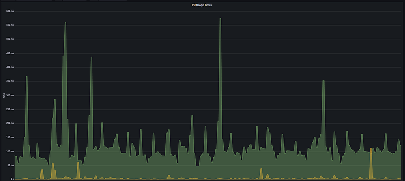
This panel measures the amount of time the disk is actively engaged in input/output operations. High latency or busy time here is usually the primary culprit behind a general feeling of sluggishness across the system.

• The Logic: It analyzes how long the processor has to wait for a disk operation to complete. If the disk engagement time approaches 1 second per second (1000ms), it means that the disk is completely saturated.
• Critical Threshold: Sustained high values in milliseconds (ms) are definitive proof of a Disk Bottleneck (I/O Wait). Continuous spikes exceeding 100ms will lead to noticeable delays in application response times.

The PromQL Query:

irate(
  node_disk_io_time_seconds_total{
    instance="$node", 
    job="$job", 
    device=~"$diskdevices"
  }[5m]
)

Query Components:

• I/O Busy Time (node_disk_io_time_seconds_total): A counter that tracks the total time the disk spends performing I/O operations, in seconds.
• Instantaneous Latency Rate (irate): Calculates how much of each second the disk spent working during the last 5-minute period.
• Precision Monitoring: Thanks to the $diskdevices filter, we can clearly observe the pressure on the primary disk where the operating system and database reside.

Analysis Note: In the I/O Usage Times graph, very sharp spikes reaching between 550ms and 600ms are visible around 08:05 and 09:20. This indicates that, during those moments, more than half of the disk’s capacity was consumed just by I/O waits. The fact that these spikes perfectly align with the high data transfer rates in the previous Disk Throughput graph confirms that the system was hitting its disk speed limits at those times.

1.5. Network Traffic: Is the Traffic Flowing? Bottleneck Signals

This section monitors the real-time data traffic between the server, the outside world, and other microservices. By measuring the volume of data passing through the network, we can identify how much of the available bandwidth is being consumed and pinpoint potential bottleneck locations. We specifically use this data to analyze the impact of sudden traffic spikes on overall system performance.

• The Logic: Database performance isn’t just about local disk or CPU. If the network interface card (NIC) is saturated, even the fastest query will feel slow to the end-user because the results are stuck in the “network pipe.”
• The “PostgreSQL” Connection: In PostgreSQL, high network traffic is often a sign of unfiltered queries (e.g., SELECT *) or large data migrations between nodes in a cluster.

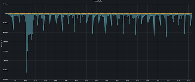
This panel analyzes the data carrying capacity of the infrastructure by measuring the amount of data passing through network interfaces per unit of time.

• The Logic: It tracks the system’s communication speed with the outside world. Sudden surges in network traffic indicate whether the system is reaching its bandwidth limits. If the traffic volume approaches the limits of the network card (e.g., 1Gbps), packet queues form, leading to latency in applications.
• Critical Threshold: If the values shown on the graph consistently approach 80% of the network hardware’s theoretical limit, it is a serious bottleneck signal. Specifically, sharp spikes like 600 Mb/s occurring within seconds indicate that the data transfer at that moment could slow down other network services.

Inbound Traffic (Incoming):

irate(
  node_network_receive_bytes_total{
    instance="$node",
    job="$job"
  }[5m]
) * 8

Outbound Traffic (Outgoing):

irate(
  node_network_transmit_bytes_total{
    instance="$node",
    job="$job"
  }[5m]
) * 8

Query Components:

• Network Data Counters (node_network_…_bytes_total): These are cumulative counters that store the total amount of data passing through the network card in bytes.
• Instantaneous Rate of Change (irate): This calculates the per-second data flow rate based on the two most recent data points within the last 5-minute window.
• *Unit Conversion ( 8):** Since the incoming data is in Bytes, the result is multiplied by 8 to convert it to Bits (Mb/s), which is the industry standard for network speed.

Analysis Note: In the Network Traffic graph, a very sharp downward spike reaching -600 Mb/s is observed in the Outbound traffic around 08:00. This proves that a very intensive data transfer was being made from the system to the outside at that moment. Other periodic spikes at the -200 Mb/s level clearly reflect the load of a routine data synchronization or backup process on the network.

1.6. OOM Killer Count: Did the OS Terminate PostgreSQL or Your Applications?

The OOM (Out Of Memory) Killer is a safety mechanism within the Linux Kernel. When physical memory is completely exhausted, the kernel forcibly terminates the most resource-heavy processes — usually PostgreSQL or Java applications — to prevent a total system crash.

• The Logic: If this metric is anything other than zero, it means your system has crossed a critical threshold where the OS could no longer manage memory and had to “sacrifice” a process to survive. For a database, this is a catastrophic event because it leads to immediate downtime and triggers a crash recovery process upon restart.
• The Risk: Even if your total RAM usage looks stable, sudden spikes in work_mem usage during complex joins can trigger the OOM Killer without warning.

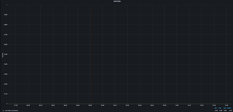
This panel tracks processes that have been forcibly terminated by the operating system due to memory exhaustion. It is one of the most critical alarm points in memory management. As seen from the graph, the OOM Killer has not been triggered during this period.

• The Logic: When physical memory (RAM) and Swap space are completely full, the operating system selects a process as a victim and kills it to keep the system from crashing. This panel analyzes how many times the kernel has triggered this mechanism. If this value is greater than zero, it is certain that the system has experienced a critical memory shortage.
• Critical Threshold: The 0 value shown in the graph indicates that no services have been killed by the operating system. Any occurrence of this event means a direct service interruption, and the tolerance threshold is zero.

The PromQL Query:

irate(
  node_vmstat_oom_kill{
    instance="$node", 
    job="$job"
  }[5m]
)

Query Components:

• OOM Kill Counter (node_vmstat_oom_kill): A counter that maintains the total number of OOM Killer events since the system was booted.
• Instantaneous Increase Rate (irate): Checks if there has been an increase in this counter during the last 5-minute period. An increase in the counter indicates that a process was killed within that time window.

Analysis Note: In the OOM Killer graph, the value is observed at the 0.00 level throughout the entire time range. The metric values (min, max, avg, current) are all zero. This proves that no processes were terminated by the operating system due to memory insufficiency during the analyzed period. System memory currently remains within safe limits.

1.7. Uptime & Stability: System Continuity

This panel tracks how long the system has been running without a reboot. While high uptime is often seen as a badge of honor for stability, in a monitoring context, it serves as a critical diagnostic tool to detect unscheduled reboots or “silent” crashes.

• The Logic: It measures the time elapsed since the last kernel boot. If the uptime value suddenly resets to zero, it indicates the server has restarted — potentially due to a power failure, a kernel panic, or a manual intervention.
• Stability Analysis: Constant reboots (low uptime) are a major red flag for hardware issues or critical software conflicts. Conversely, extremely high uptime (years) might suggest the system is missing vital security patches or kernel updates that require a restart.

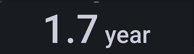
This panel measures exactly when the server was last rebooted and how long it has been providing uninterrupted service. It is a fundamental indicator of the system’s stability and operational continuity.

• The Logic: It calculates the total running time (uptime) of the system. While long-term uptime values generally point to a stable operating system and hardware infrastructure, unexpectedly low uptime values prove that the system has experienced a crash or an unplanned reboot.
• Critical Threshold: Rather than a specific “threshold” value, we monitor for sudden drops in this panel. If the uptime duration suddenly resets to zero, it indicates the server was restarted due to a kernel panic, hardware failure, or manual intervention. In critical environments, this value is expected to be in the range of months or even years.

The PromQL Query:

node_time_seconds{instance="$node", job="$job"} 
- 
node_boot_time_seconds{instance="$node", job="$job"}

Query Components:

• Current Time (node_time_seconds): Provides the current Unix timestamp of the server in seconds.
• Boot Time (node_boot_time_seconds): Holds the Unix timestamp of the moment the operating system last started.
• The Calculation: By subtracting the boot time from the current time, we find out for how many seconds the system has been up. Grafana automatically converts this into years, months, days, or hours.

Analysis Note: The Uptime panel in the visualization shows that the system has been running continuously for 1.7 years. This demonstrates that the server and the services running on it (PostgreSQL, etc.) are incredibly stable, having gone approximately 620 days without any critical crashes or reboots required for updates or repairs. This is a clear testament to enterprise-level High Reliability.

Section 2: PostgreSQL Engine and Cache Efficiency

This section focuses on the heart of performance: how fast data is retrieved. The moment a database is at its fastest is when it accesses data directly from memory (RAM) instead of the disk.

• The Core Concept: Every time a query is executed, PostgreSQL first looks for the data in its own Shared Buffers. If it’s not there, it checks the OS Page Cache. If it’s still not found, it must perform a costly “Physical Read” from the disk.
• The Performance Goal: Our objective in this section is to minimize disk I/O. We will analyze the Cache Hit Rate to see how often we successfully avoid the disk and monitor Temp File Usage to catch queries that are “spilling” over into the storage layer.

2.1. PG Buffer Cache Hit Rate: Why is 99% the Golden Standard?

The Cache Hit Rate is the most vital health indicator for a PostgreSQL instance. It represents the percentage of data requests handled by the RAM.

• The Logic: If your hit rate is 99%, it means only 1 out of every 100 requests actually touches the disk. If this drops to 90%, your database could feel 10x slower because disk latency is magnitudes higher than memory latency.
• The “99%” Rule: For OLTP (transactional) workloads, anything below 99% usually indicates that your shared_buffers are too small for your "hot" data (the data accessed most frequently).

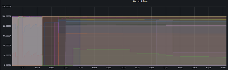
This panel measures the percentage of data requests satisfied by the RAM versus those that require a physical Disk Read. It is the ultimate metric for database speed.

• The Logic: A database is at its peak performance when it finds data in the Shared Buffers (RAM). This panel calculates the success rate of these “memory hits.”
• Mathematical Logic: The total amount of hits is divided by the total number of reading attempts (hits + reads) to obtain a percentage success rate.

The PromQL Query:

pg_stat_database_blks_hit{instance="$instance"} 
/ 
(
  pg_stat_database_blks_read{instance="$instance"} 
  + 
  pg_stat_database_blks_hit{instance="$instance"}
)

Query Components:

• blks_hit: The number of blocks that the database successfully read directly from memory (shared buffers) instead of the disk.
• blks_read: The number of blocks that were not found in memory and had to be fetched from the disk.
• Success Ratio: This formula identifies how much of your workload is “memory-resident.”

Analysis Note: In the Cache Hit Rate graph, most databases are seen hovering at 90% and above, which is generally healthy. However, certain services at the bottom (represented by the green and purple lines) operating in the 20–40% band prove that these specific tables or queries are failing to use memory efficiently. This indicates a high probability of Disk I/O bottlenecks. Key Takeaway: If this ratio is consistently low, you must either increase the shared_buffers parameter or optimize "expensive" queries that perform excessive disk reads.

2.2. Temp File Usage: Traces of Memory Spills

In PostgreSQL performance analysis, Temp File Usage is one of the most critical signals indicating that the database is “running out of breath.” When queries cannot fit into the allocated memory and spill over to the disk, performance drops dramatically.

• The Logic: For operations like sorting (ORDER BY), joining (HASH JOIN), or creating indexes, PostgreSQL uses a memory area called work_mem. If the data required for these operations exceeds the work_mem limit, PostgreSQL creates temporary files on the disk to process the data.
• The Performance Impact: Because writing to and reading from disk is significantly slower than RAM, a query that generates large temp files will take much longer to complete and will put an unnecessary burden on the I/O subsystem.

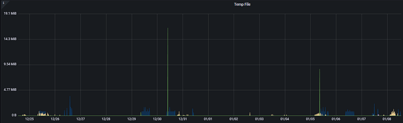
This panel measures how much temporary space PostgreSQL is using on the disk to perform operations. Ideally, we want all operations to be completed in RAM; however, in certain scenarios, the database is forced to create temporary files.

• Why do queries spill to disk? If the memory required for a SORT, HASH JOIN, or DISTINCT operation exceeds the work_mem limit configured in PostgreSQL, the database begins using the disk to complete the task. Since disk access is significantly slower than RAM, this can turn sub-second queries into multi-minute nightmares.
• Analysis: Looking at the Temp File graph, we see sudden spikes reaching approximately 17 MiB and 9 MiB on 12/30 and 01/05. These spikes prove that a “heavy” or inefficiently written query — attempting to sort massive datasets — was executed at those specific moments.

The PromQL Query:

irate(
  pg_stat_database_temp_bytes{
    instance="$instance"
  }[5m]
)

Query Components:

• temp_bytes (pg_stat_database_temp_bytes): A counter that tracks the total amount of data written to temporary files by a database in bytes.
• Instantaneous Rate of Change (irate): Calculates how many temporary files are being created per second over the last 5 minutes. This is the most sensitive method for catching instantaneous bottlenecks.
• Filtering ($instance): Allows us to pinpoint exactly which database instance is experiencing the issue.

Recommendation: If you see constant or very high spikes in this graph, you should consider increasing the work_mem parameter to a safe level or optimizing the queries triggering these spikes (e.g., by adding missing indexes).

Bu bölümü, uygulama katmanı ile veritabanı arasındaki kritik köprüyü ve bağlantı yönetiminin performans üzerindeki etkisini vurgulayan profesyonel bir üslupla İngilizceye çevirdim.

Section 3: Traffic, Connections, and Timed Risks

This section analyzes not just the hardware level, but how your database interacts with the application layer. Managing how many users and applications connect to your database is vital for maintaining stability under high load.

3.1. Active vs. Idle Sessions: Connection Management

Connection management is the art of balancing resources. Every connection made to PostgreSQL consumes memory and CPU; therefore, having too many “waiting” or “stuck” connections can be just as damaging as a heavy query.

This panel tracks the number of clients that are actually executing a query at any given millisecond. It is the most direct measure of the “concurrency” pressure on your database.

• Is 100 Active Sessions a lot? In a PostgreSQL environment, 100 truly active sessions is a significant load. Since each active session typically maps to a CPU thread, having 100 concurrent queries on a server with fewer CPU cores leads to context switching and performance degradation.
• The “Peak” Risk: While the system might handle a baseline of 10–20 active sessions comfortably, hitting a spike of 100 active connections simultaneously can saturate the CPU and cause a massive spike in query latency.

Analysis: In the Total Active Sessions graph, the data points generally stay at a manageable baseline. However, at a specific point — likely during a batch job or a complex reporting window — we see a vertical surge hitting 100 active sessions. These spikes are “danger zones” where the risk of reaching the max_connections limit is highest. If this 100-session threshold is hit frequently, it’s a clear signal that the application is either not closing connections fast enough or the database needs more CPU "runway" to process tasks faster.

The PromQL Query:

sum(
  pg_stat_activity_count{
    datname=~"$datname", 
    instance=~"$instance", 
    state="active"
  } != 0
)

Query Components:

• pg_stat_activity_count: This is the foundational metric that tracks the state of every session currently connected to the database.
• state=”active”: It filters the data to show only the connections that are actively executing a SQL command at this very moment.
• sum: Aggregates data from different database instances, providing a single, unified number for the total active workload.
• != 0: A filter that ensures only records with actual activity are processed, effectively filtering out “silent” or non-reporting instances.

Analysis Note: If the number of active sessions is low (e.g., under 10) yet users are still reporting significant sluggishness, the problem is likely not the volume of connections. Instead, it indicates that those few running queries are stuck waiting for Disk I/O or are blocked by Table Locks. This metric helps you distinguish between a “traffic jam” (too many queries) and a “roadblock” (stuck queries)

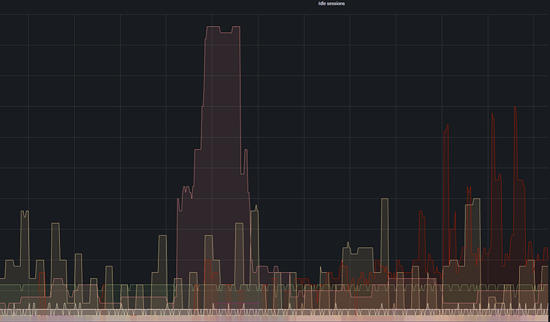
This panel measures the density of sessions that are connected to the database but are currently performing no work. In PostgreSQL, since every connection is a separate operating system process, these sessions continue to consume memory even when they are doing nothing.

• Is 500 Idle connections a risk? Yes. Idle connections bring you closer to the max_connections limit, potentially preventing new “active” tasks from entering the database. Furthermore, connections in the “idle in transaction” state can hold onto database locks, effectively paralyzing parts of the system.
• When is PgBouncer needed? If your Idle Sessions graph (shown as the large red and yellow areas in the visual) is consistently much higher than your Active Sessions, implementing a connection pooler like PgBouncer will typically increase system performance by 30–40%.

Analysis: Looking at the Idle Sessions graph, a massive red block (representing a high number of idle connections) is visible during a specific central time frame. This proves that the application is connecting to the database but failing to close the connection after the task is finished, indicating inefficient connection management.

The PromQL Query:

pg_stat_activity_count{
  datname=~"$datname", 
  instance=~"$instance", 
  state=~"idle|idle in transaction|idle in transaction (aborted)"
}

Query Components:

• pg_stat_activity_count: The core metric that counts the states of database sessions.
• State Filtering: This covers three different “idle” states:
• idle: The connection is open, but no work is being done.
• idle in transaction: A transaction has started (BEGIN) but has not been finished (COMMIT/ROLLBACK). This is the most dangerous state as it causes locks and prevents vacuuming.
• idle in transaction (aborted): A transaction that encountered an error but remains open.
• Scope: Uses $datname and $instance variables to allow for specific database-level analysis.

Analysis Note: The large fluctuations in the graph indicate an imbalance in the application’s Connection Pooling logic. Persistently high “Idle” values cause the database server to use unnecessarily high amounts of RAM, which could be better utilized by the Buffer Cache.

3.2. Database Size & Growth: Data Distribution and Trends

This section covers the capacity planning and storage management pillar of our PostgreSQL analysis. It allows us to understand the physical footprint of your data and identify long-term growth trends.

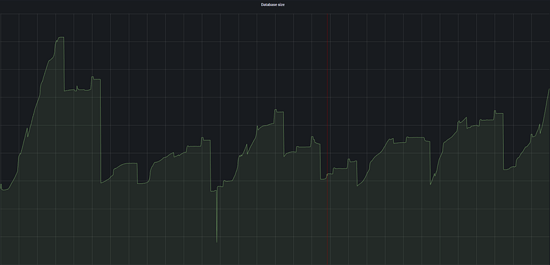
This panel displays real-time changes in the size of selected databases and their usage patterns.

• The Logic: It analyzes not just how large the database is, but how aggressively it writes or deletes data.
• Analysis: The sawtooth (up-and-down) patterns in the graph indicate heavy usage of temporary data. Sharp drops are usually the result of VACUUM operations, table truncates, or large batch DELETE operations. This fluctuating structure proves that the database is not a static warehouse but a living engine that constantly cleans itself.

The PromQL Query:

pg_database_size_bytes{
  datname=~"$datname", 
  instance=~"$instance"
} 
/ 1099511627776

• Query Components:
• pg_database_size_bytes: Fetches the total physical size (data + indexes) on disk in bytes.
• Conversion Factor (1099511627776): The mathematical value to convert Bytes to Terabytes (1024⁴).
• Dynamic Filtering: Enables tracking the total load of a single database or the entire cluster in TB.

This panel shows the long-term trend of the total data load on the server in Terabytes (TB).

• The Logic: Monitoring database sizes at a higher scale (TB) provides a strategic perspective on disk occupancy.
• Analysis: The nearly horizontal lines in this graph indicate that database growth is under control. This is the most reassuring graph for infrastructure teams; it documents that the data increase rate does not threaten disk capacity in the short term and that growth is linear and predictable.

The PromQL Query:

topk(5, 
  pg_database_size{instance="$instance"}
)

• Query Components:
• Unit Conversion: While the first query captures real-time fluctuations in Bytes, this query shows the “big picture” by scaling to TB.
• Top 5 (topk): Filters out noise by focusing only on the top 5 databases putting the most pressure on the disk.
• In Summary: The first table answers “What is the database doing right now?” (maintenance or intensive writing), while the second table answers “When will the disk be full?”

3.3. Replication Lag: High Availability (HA) Analysis

Replication Lag measures the synchronization delay between the Primary database and its Replica.

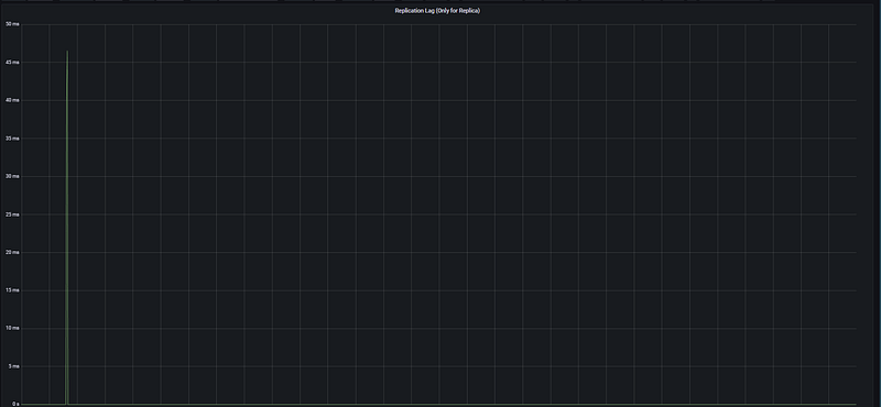
This is the primary indicator of potential data loss during a disaster recovery scenario.

• Instantaneous Spike: A sharp spike of ~47 ms is visible around 07:45. This represents a momentary delay during the transmission of an intensive write operation from the primary to the replica.
• System Stability: The fact that the value returns to 0 ms immediately after the spike proves that the replica’s catch-up speed is very high.
• Overall Health: The flat line in the rest of the graph indicates maximum data consistency and near-zero risk of data loss in case of a disaster.

The PromQL Query:

rate(
  pg_replication_lag{
    instance="$instance"
  }[5m]
)

• Analysis Note: If this value climbs from milliseconds to seconds (e.g., >10s), it signals network bandwidth issues or hardware insufficiency on the replica server.

Section 4: Bottlenecks, Deadlocks, and “Rogue” Queries

Analyzing database performance only through resource usage (CPU/RAM) can be misleading. In this section, we analyze edge cases that slow down the system from within and cause the engine to be unnecessarily busy.

4.1. Longest Transaction & Top Long-Running Queries

This panel tracks the longest-running active transactions in the database. Long transactions not only consume resources but also block VACUUM processes, leading to table bloat and locks.

• Why Monitor This? A very long transaction usually points to an inefficient query, a missing index, or a connection left open by the application (idle in transaction).
• Graph Interpretation: The vertical orange lines represent periodic spikes in transaction duration. These prove the impact of background Batch jobs or reporting queries on the system.
• Optimization Step: Queries exceeding a threshold (e.g., 30 seconds) should be examined with the EXPLAIN ANALYZE command to identify bottlenecks like Sequential Scans.

The PromQL Query:

pg_stat_activity_max_tx_duration{
  instance="$instance"
} > 0

4.2. Lock Tables: Contention Analysis

Lock Tables allow us to detect situations where database operations block each other, potentially bringing the system to a standstill.

• Why is Locking Dangerous? When a transaction locks a table, all other operations trying to access it must wait. If the lock isn’t released, this queue grows until it hits the max_connections limit, locking the entire system.
• Graph Interpretation: The numerous thin, vertical red spikes indicate frequent, short-term locking. If these coincide with Longest Transaction spikes, queries must be accelerated or transaction windows shortened to reduce contention.

The PromQL Query:

pg_locks_count{
  datname=~"$datname", 
  datname!="postgres", 
  instance=~"$instance", 
  mode=~"$mode"
} > 1

Section 5: Conclusion and Action Plan

Following the detailed analysis, the following steps must be implemented to ensure continuity in both the infrastructure and database layers.

5.1. Quick Wins: 3-Step Performance Improvement

If the analysis detects a Low Cache Hit Rate or Long-Running Queries, these immediate actions will boost performance:

1. Memory Optimization (Shared Buffers): If the Cache Hit Rate is below 99%, increase PostgreSQL RAM allocation capacity by adjusting the shared_buffers parameter.
2. Query and Index Revision: Examine the Longest Transactions using EXPLAIN ANALYZE. Reduce the Disk I/O load by adding appropriate indexes to tables performing a Sequential Scan.
3. Temporary File Control: If there is a spike in Temp File Usage, increase the sorting memory allocated for each session (work_mem) to prevent operations from spilling over to the disk.

5.2. Monitoring Strategy: Critical Alert Thresholds

To catch problems before they escalate without constant manual supervision, the following Alerting rules should be defined on Grafana or Prometheus:

+-----------------------+-----------------------+------------------------------------------+
| Metric                | Critical Threshold    | Description / Action                     |
+-----------------------+-----------------------+------------------------------------------+
| CPU Busy              | > 85% (for 10 min)    | Check for Scaling needs.                 |
| Filesystem Usage      | > 90%                 | Perform log cleanup or expand the disk.  |
| OOM Killer            | > 0                   | Urgent! RAM exhausted, OS killing tasks. |
| PG Cache Hit Rate     | < %95                 | Query optimization or RAM upgrade.       |
| Replication Lag       | > 10 seconds          | Check replica sync and network.          |
| Idle in Transaction   | > 5 minutes           | Terminate (kill) abandoned connections.  |
+-----------------------+-----------------------+------------------------------------------+

General Evaluation

PostgreSQL monitoring is not just about glancing at graphs; it is the art of reading the correlation between them. As seen in this guide, a rise in CPU might not mean much on its own; however, when combined with high IOPS and Temp File Usage, it clearly signals an inefficient sort operation that does not fit in memory and is exhausting the disk.

Database performance is not a static state, but a process in constant motion. For a healthy PostgreSQL ecosystem:

• Observe: Monitor both operating system and database metrics from a single, unified panel.
• Set Thresholds: Deploy Alerting mechanisms before issues impact the end-user.
• Optimize Continuously: Periodically analyze the Longest Transactions and Locks to prevent technical debt from accumulating.

Remember: in a well-monitored system, no slowdown is meaningless. The right metrics will always illuminate the path to the root cause.